


An Economic Simulation of the Path to Sustainable Energy: A Dynamic Analysis
| Charles Mason 1 , 2 ,* ,Rémi Chassé 3 |
| 1 Department of Economics and Finance, University of Wyoming, Laramie, USA |
| 2 Grantham Research Institute, London School of Economics, London, UK |
| 3 Department of Economics, University of Prince Edward Island, Charlottetown, Canada |
* Corresponding author. |
1.- Introduction
For roughly 50 years, economists have debated the concept of sustainability [1]. Much of this literature interprets sustainability as non-decreasing well-being of a typical member of society [2]. To operationalize this concept, much of the existing economic literature employs economic growth models, and adapts the associated results on capital accumulation and resource use to “real-world” data [3]. A general finding is that for future generations to be at least as well off as current generations, society must invest the rent from non-renewable resource use to increase the stock of physical capital [4]. When consumption of a non-renewable resource is associated with pollution, as with fossil fuels, society is motivated to transition to an alternative, more sustainable, resource.
In general, economists have modeled this sort of transition by contrasting resource use from a non-renewable source against the use of a “backstop” technology. The backstop is usually assumed to be able to deliver any amount of energy at a constant marginal cost, which implies the resource use can be expanded to the extent society desires without increasing its marginal cost. For many renewable resources however, the associated marginal cost of production is zero, or close to zero. Most of the costs associated with renewable energies are sunk; it is expensive to build the capacity to generate energy from renewable resources [5, 6]. This generating capacity then constrains the amount of renewable energy that is available; to increase renewable resource use, capacity must be expanded.
In this paper, we address this inconsistency in the existing literature by presenting a model that more satisfactorily characterizes the role of renewable energy. Our model focuses on the role energy plays in society's potential to produce goods and services. As with much of the existing literature, energy can be allocated to output production or pollution abatement; our extension allows energy to be invested in the development of renewable resource capacity [7, 8]. We also allow for capacity changes to depend on the stock level, which could reflect learning-by-doing. Working against any increases in capacity is wear and tear from the use of the renewable energy [9, 10]. In this way, our model provides a more satisfactory characterization of the role played by renewable energy in the time path of the typical individual's well-being, and hence the implications for sustainability, than can be found in the extant literature.
The paper is organized as follows. We start in section 2 by reviewing the relevant literature. In section 3, we discuss our model, emphasizing natural resources, the production of energy and its different uses. In section 4, we present a numerical simulation of the model in section 5. We offer some discussion in section 6, and conclude in section 7.
2.- Literature Review
The publication of Meadows et al.'s [11] book Limits to Growth triggered a strident response by mainstream economists [12, 13]. Nordhaus [14], for instance, points out the dynamic complexities of the mathematical model and more importantly, criticizes the lack of human behavior in the original book and subsequent iterations, particularly responses to economic scarcity. The general spirit was to refocus the debate concerning “sustainability,” which has typically been interpreted as the requirement that a typical member of society does not suffer decreasing well-being [1, 2, 15]. Later, inquiries into the sustainability of coal consumption created a firm link between questions of sustainability, however defined, and energy consumption.
In thinking about sustainability, one is naturally led to a consideration of patterns of possibilities over time. The focus in this paper is on human values, as we are economists and that is the nature of economic analysis. The human values in question generate a level of aggregate well-being, or satisfaction; we refer to this as “felicity” in the pursuant discussion, and denote it by . We interpret “sustainability” as the requirement that felicity never declines [1, 16].
There is a conceptual link between sustainability and the use of a non-renewable resource whose usage generates pollution [17, 18]. For future generations to be at least as well off as current generations, society must carefully consider the inter-temporal evolution of consumption and resource use. To achieve a sustainable outcome in this situation, society must invest the rent from non-renewable resource use to increase the stock of physical capital [4]. When consumption of a non-renewable resource is associated with pollution, society is motivated to lower its use of that resource [19]. This motivates a transition to an alternative, more sustainable, resource.
When pollution is linked to non-renewable energy use, the associated social costs are accounted for; this can lead to a phase where both resources are used simultaneously, even though non-renewable energy and the clean alternative (the “backstop”) are perfectly substitutable [20]. This feature is also observed by Jouvet and Schumacher [21], who link the time of the switch to the economy's level of man-made capital. At that moment, society has depleted its natural resource stock, with no potential for simultaneous use. Switching too early would imply forgoing low-cost energy, which helps boost the economy and increases consumption.
Simultaneous use can also occur when the marginal cost of the renewable backstop is increasing. When both the energy demand and the cost of renewable energies are low, society may use renewables only first, then switch to simultaneous resource use before switching again to renewables in either finite or infinite time. Some non-renewable energy stock may be left in the ground, implying a phase in which the economy only uses renewable energies [22].
Van der Ploeg and Withagen [23] link the initial levels of capital, pollution and non-renewable resource stock to the type of energy used and the order in which they are used. They find that simultaneous energy usage always follows an oil-only economy and only happens as man-made capital is above its carbon-free steady-state level. Oil is never phased out and man-made capital has to be reduced to reach its long-run level; the oil-only economy “overshoots.” According to this view, simultaneous use occurs as the man-made capital stock is drawn down. As society currently is using both renewable and non-renewable energy, their model would require society to be in the process of lowering man-made capital to reach the carbon-free steady-state level, which seems at odds with the real-world.
As we noted above, generating energy from renewable sources is typically constrained by the installed capacity at any given time. In the presence of such constraints, it is entirely possible that there will be a period when both types of resource are used simultaneously. Expanding the renewable capacity would ease this constraint, leading to a period in which the share of renewable resource use rises over time, as society transitions away from the non-renewable resource base.
Such a pattern is fully in line with reality: for example, over the past decade the role of coal in producing electricity in the United States has been steadily shrinking, while the share attributable to wind and solar energy has been rising. Moreover, the presence of capacity constraints implies the need to introduce a second state variable, measuring capacity; this feature is absent from all the papers discussed above. A key innovation in this paper is the introduction of this second form of capital.
3.- An Economic Model
In this paper we adopt a neoclassical economic growth model, and use a “Capital Approach” to sustainability [24]. Our point of departure regards the role energy plays in society's potential to produce goods and services, and the manner in which that energy is itself produced.
We envision a world with two types of energy producing resources. One type of resource is non-renewable; one can think of conventional fossil fuel as a good example. The other type of resource is renewable, for example wind and solar power, or biofuels. We denote the non-renewable resource stock as and the renewable resource capital stock . While our conceptualization of a renewable resource is related to the concept of a “backstop technology” in the extant literature, these papers typically assume the backstop will be fully available—i.e., society has access to whatever quantity of the resource as it wishes to use at a given time. We believe this fails to capture a key element: that society must first invest in renewable natural capital before it can access renewable energy.
Society can generate energy through the rate of use of non-renewable natural capital and renewable natural capital. Henceforth, we will refer to the flow of non-renewable natural capital used as “extraction,” and denote it by ; we refer to the flow of renewable natural capital used as “harvest,” and denote it by . The quantity of energy produced is described by the energy transformation function
This energy can be allocated to multiple uses, including pollution abatement, output production and renewable resource development. While both non-renewable and renewable resources are capable of producing energy, one is relatively abundant (at least initially) and relatively dirty, namely the non-renewable source.
Extraction of non-renewable capital subtracts from the stock of the non-renewable natural capital . This evolution through time is described by the differential equation [25]:
Renewable energy is generated by exploiting a renewable natural capital. We also think of the capital as a capacity: although renewable energies— wind, solar, hydro or biomass—are readily available, one needs to invest in this capacity before society can capture the renewable energy [26]. Investment in this capacity is based on the share of total energy that is allocated to it, where . We denote the relation between investment in the renewable resource stock and this allocation of energy by the function . Although the marginal cost of renewable energies is zero, the cost of the investment in existing capacity is the lost benefits associated with allocating energy to other valuable uses. Using renewable energies causes wear and tear, which causes depreciation [27, 28]. We include that feature by explicitly having the capacity depreciating with the use of the renewable resource, as measured by . Accordingly, the rate of change in is summarized by the following state equation:
Non-renewable natural capital can be thought as a measure of the aggregated stock levels of fossil fuels, or other resources that can be used to produce energy, for example uranium. While extraction of non-renewable natural capital generates non-renewable energy, it also entails environmental degradation. Tailings piles, the accumulated residue from mineral extraction, are a prime example. These stockpiled residues decrease utility by their mere presence and may also introduce hazardous mineral elements into the environment [29]. Petroleum extraction is associated with high levels of carbon emissions, and the use of petroleum-derived products can lead to air and water pollution. Another example is the presence of floating patches of discarded plastic in northern and southern Atlantic and Pacific oceans and in the Indian ocean; they pose threats to wildlife and marine ecosystems [30]. In addition, environmental pollution from certain chemicals used in resource extraction can accumulate in the environment and cause disutility.
We interpret these adverse environmental effects as arising from a stock of “pollution”, which we denote by . We assume that pollution is an increasing, convex function of non-renewable resources extraction . Mitigating this pollution requires the expenditure of effort and energy into “abatement” . Letting represent the share of energy directed into abatement, we write the level of abatement as . Altogether, then, the evolution of the pollution stock is described by:
Felicity depends on the flow of aggregate consumption, , as well as the effective capacity of renewable resources to produce energy —which we often refer to as “renewable natural capital” in the pursuant discussion —and the stock of pollution, . The production of goods and services also opens up the potential to increase the stock of what we refer to as physical capital, , itself an important input into the production process. The amount society invests in physical capital equals the difference between output, , and consumption, . Because all output will be consumed or invested, we need only discuss one of the two; here, we focus on the optimal time path of consumption. Physical capital is prone to depreciation, at the rate , so that the evolution of the physical capital stock is described by the differential equation:
By adding to physical capital, current generations can create a potential offset to accumulated pollution, which might then allow future generations to enjoy a level of well-being at least as large as that of the present. But as the non-renewable natural capital stock is drawn down, actions must be taken to facilitate its replacement, by building up the renewable natural capital stock.
In a conventional growth model, society allocates output to consumption or investment. In our interpretation, energy—a key input into the production function that generates output—is directed to productive purposes or to increase the effective renewable natural capital stock. One can think of energy as facilitating maintenance, which serves to offset some of the depreciation that arises from use of windmills or solar panels (as discussed in [6]), or as investment into new structures. These efforts can either be helped or hindered by the level of existing stock of renewable resources [27, 31].
We envision a central decision-maker, or “social planner,” who is charged with promoting the well-being of society for all time. The social planner evaluates the level of felicity at every moment, weighting each contribution depending on the time at which the felicity is generated. In this regard, she uses an inter-temporal social discount rate, [32, 33, 34]. The social planner's task is to select a time path of consumption level, energy allocation and resource uses so as to maximize the discounted flow of felicity over an infinite horizon. The planner's decision problem is constrained by equations that describe the evolution of the capital stocks.
4.- Numerical Simulation
To focus on the broader features of our model, we conduct a numerical simulation [35, 36]. To operationalize this simulation, we start by specifying the various functional forms in the model.
Given the chosen parameters and functional forms, society gradually shifts from using non-renewable to renewable energies, eventually abandoning the use of the former. This transformation occurs even though the non-renewable resource is still plentiful. Accordingly, we split our discussion between the phase where non-renewables are used and the phase after their use ends. A particular focus of our analysis of the post non-renewable resource phase is its long term equilibrium and stability. Modelling the effective capacity of renewable resources to produce energy as a state variable, and capturing capacity constraints, impacts this long run equilibrium. For the steady-state level of renewable resource to be positive, society has to be relatively averse to intergenerational inequity.
We assume the utility function is non-separable in consumption , the renewable resource stock and pollution stock [37, 38], with [39, 40]:
The ratio of over can be thought of as a sort of “green index”. For instance, if is measured in units of generated from non-renewables and is the concentration level, would represent the fraction of avoided emissions associated with the use of renewable energies.
A key feature of our model is the presence of two types of energy, non-renewable and renewable energies. We adopt the linearly additive energy-generating function:
so that renewable and non-renewable resources are perfect substitutes in the total generation of energy.
We set the functional relation between energy investment and renewable resource capital as so that energy increases renewable natural capital, but at a decreasing rate. the functional relation between energy and abatement as . We assume the relation between non-renewable resource extraction and contributions to the pollution stock is given by . Finally, we set the depreciation rate of physical capital at , and the discount rate equal to .
Noting that the share of energy allocated to production is , we define the amount of energy allocated to production as . We assume a production function of the form . Hence, capital and energy are imperfect substitutes; there can be no output without some energy as an input. Following van der Ploeg and Withagen [23], we chose and .
4.1.- Simultaneous Use
We start off by analyzing a scenario in which society initially uses both resources; after time, society may switch completely into green energy [41].
Over time, the use of non-renewable energies decreases as society gradually switches to renewable energies. Since extraction of non-renewable physical capital is initially positive, the associated stock decreases until time , where falls to zero. In this particular simulation, non-renewable energies become virtually irrelevant by [42]. This represents a corner solution which is an interesting feature in economic growth models: it may become optimal to completely stop using non-renewable energy and in favor of sustainable energy from renewable resources. The fact that this path involves such a corner solution is a direct consequence of the perfect substitution between the two natural resources.
The shares of energy allocated to renewable natural capital and abatement decrease over time, implying that the share allocated to output increases. These effects are mirrored in the paths of total energy allocation. While there is a monotonic decrease in the use of non-renewable energies, this need not preclude growing felicity as Figure 1 illustrates: In our simulation, switching to renewable energies is associated with continuously expanding felicity and consumption over time.
At time , the values for each state and controls are: ; ; ; ; . In the pursuant discussion, we use values similar to these to illustrate how society can achieve a long-run stable outcome.
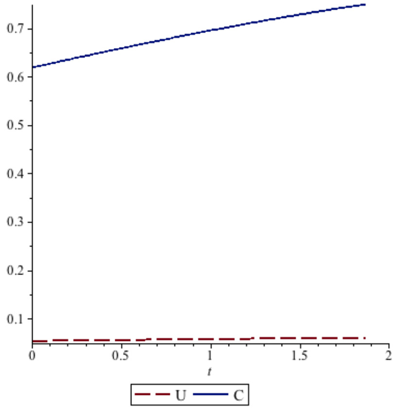
Figure 1. Felicity and Consumption.
We now analyze the effect of variations in the discount and capital depreciation rates, as well as variations in the initial values of pollution and renewable resource stock, on the time of the switch toward renewable resources. As in [23], we find that increasing the discount rate (here, from to ) postpones the time of the switch (from to ). A higher discount rate implies that the future is discounted more, and hence is less important in today's decision. This induces a postponement of the switch to renewables, since the discounted costs from higher future pollution are given smaller weight.
An increase in the rate of depreciation of capital also leads to a postponement of the switch. When increases from to , increases from to . Since capital depreciates faster, society must increase its use of non-renewable resources to compensate for lower future capital stocks.
Altering the initial values of and also lead to different scenarios. A lower initial level of pollution (e.g., instead of ) would also postpone the time of the switch to renewables (from to ). As society has a distaste for pollution, lower levels of permit longer extraction of non-renewables.
An increase in the initial stock of renewables, e.g. raising from to of the steady-state value of , would induce society to suspend its use of renewables altogether at . But this suspension can only be temporary, as the disutility from pollution will increase ever-more rapidly, while the stock of non-renewables will decrease more rapidly. Accordingly, at some point in the future, society will start resume its use of renewable energies, possibly alongside non-renewables before phasing the latter out [20]. Given the exhaustible nature of the non-renewable natural capital, society must ultimately fully switch to using renewable resources.
4.2.- The Post-Non-Renewables Phase
We now turn to the phase in which society is no longer using non-renewables—a situation that some might regard as a sustainable outcome. During this phase, society could still be abating pollution from previous non-renewable resource use, with ; this will depend upon society's distaste of pollution.
Given our functional forms, it is possible to find analytical solutions for the steady-state values in this phase. Based on the chosen parameters, one may determine the steady-state values of each relevant state and control variables [43]: ; ; ; ; . For society to reach that steady-state, the path it selects must follow the stable branch after society stops using the non-renewable resource [44].
Following [23], we set the initial level of physical capital equal to one half its steady-state level. In figures , , and , we plot the time trajectory of each state and control variable, with the top horizontal line in each figure representing their respective steady-state level. With the exception of , all variables approach the steady-state monotonically from below.
Figure 6 shows the stable trajectories for felicity , capital and the renewable resource stock for five scenarios; the steady-state is represented as the black dot in the centre. The trajectory identified by circles shows the case for which both and are each half their steady-state value, which we refer to as “scenario (i)” in the discussion below. Figure 6 also includes trajectories corresponding to the following scenarios: scenario (ii) sets and ; scenario (iii) sets and ; scenario (iv) sets and . Trajectory (v) starts at the off-center diamond, which corresponds to values of the state and control variables close to those obtained at in the simulation from Section [45]. This point shows an unsustainable level of utility, as consumption , harvest and the share of energy to output are all too high when compared to the their values should society be on the stable arm leading to the steady-state. Because the levels of and cannot be instantaneously adjusted, society has to lower consumption C (from to ) and renewable resource use (from to ). This adjustment allows society to redirect some energy to increasing renewable natural capital, by reducing (from to ). But this shift causes a one-time loss in felicity, as represented by the arrow on the graph [46].
As Figure 6 illustrates, any trajectory starting from initial values of and that are larger than their steady-state value would imply that felicity declines at some point. Thus, only scenario (i) is sustainable; the other scenarios represented in Figure 6 are not sustainable. Thus, a necessary condition for sustainability is that the initial values of and are smaller than the corresponding steady-states. But there are trajectories with a small initial value of that is not sustainable, so the condition is not sufficient. We illustrate the point in Figure 7: there, we see that for some values of below the steady-state level felicity decreases for a period (though it ultimately would increase as we moved closer to the steady-state).
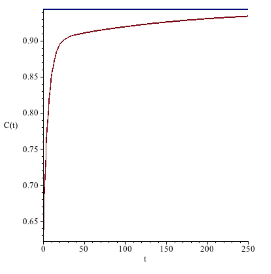
Figure 2. Consumption.
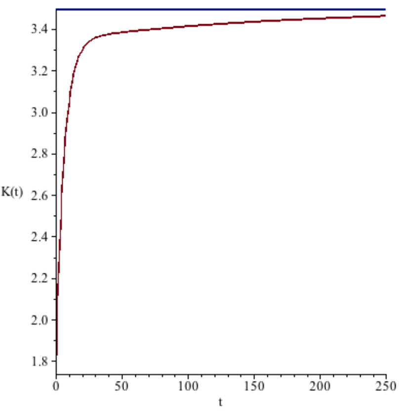
Figure 3. Capital.
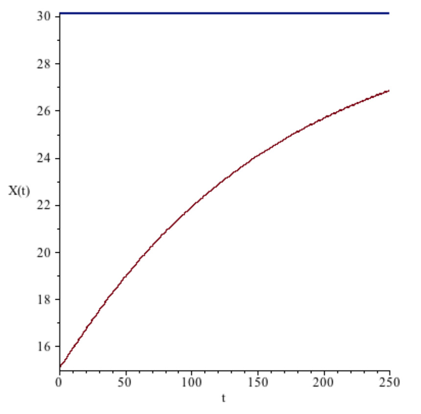
Figure 4. Renewable Resource.
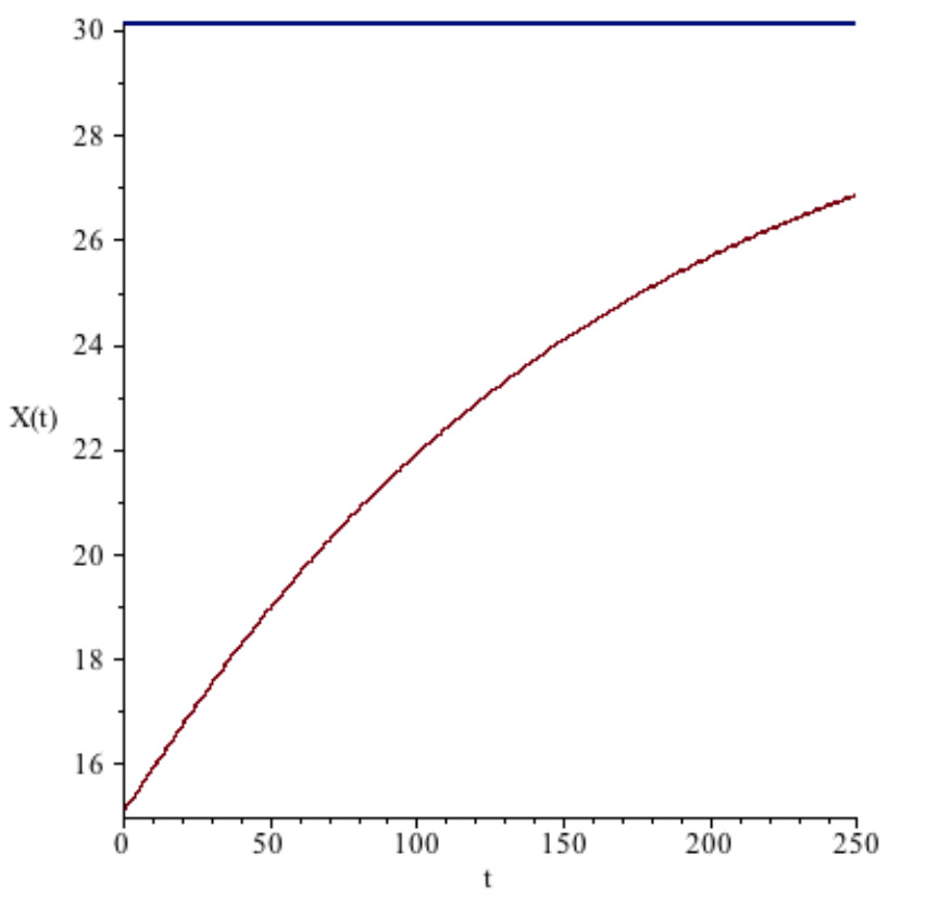
Figure 5. Energy Share to Output.
4.3.- Policy Simulation
In this sub-section, we provide a numerical simulation to illustrate a potential policy-relevant application of our analysis. This simulation investigates the long-run effects of a moratorium on renewable natural capital expansion. The obvious benchmark against which this simulation should be compared is scenario (v) in Figure 6. In the benchmark, it takes 69 years to be within 5% of the steady-value of capital . Hence, at : ; ; .
Imagine that for ten years, society reinvests just enough energy to maintain the initial stock of . This could be interpreted, for instance, as a moratorium put in place by a newly elected government, perhaps as a result of a decision to favor conventional energy use. The benefits of this policy are short-run increases in the levels of man-made capital and welfare; for example, the level of reached after 24 years in the benchmark scenario is reached after only 10 years under the moratorium scenario. Welfare is higher under the moratorium than in the benchmark scenario for the first 10 years. As the moratorium ends, society resumes the expansion of by increasing . This has the effect of lowering and lowers output generation , which in turn lowers consumption and felicity. But this result is inconsistent with our concept of sustainability. To reach the values of , and found at the 5% threshold of , it takes an overall of 79 years in the moratorium case, as compared to 10 years in the benchmark. The long-run effect of the moratorium is clear: A 10 year moratorium delays the time it takes to reach by 10 years. Because society derives welfare from renewable natural capital—it is a valuable asset to society—it is better for society to start investing in it straightaway, as opposed to delaying for a period of time.
4.4.- Imperfect Substitution Between Energy Inputs
Our numerical simulations assumed perfect substitution between renewable and non-renewable resources in energy generation. In practice, renewable energies are subject to intermittency and storage constraints which can inhibit substitution. That said, one would expect that it is possible to produce some energy even if [47]. For it to be possible to generate energy if society no longer relies on non-renewable resources, i.e. , one of two scenarios would obtain: Either non-renewable capital would be exhausted in finite time, as in Section , or society would have to manage its use of both types of natural capital so as to asymptotically converge to the post non-renewable resource steady-state. In the second situation, non-renewable resources would be gradually phased out in favor of their renewable alternative. Thus, the steady-state values of physical and renewable natural capital, consumption and energy shares correspond to post non-renewable regime we discussed above, whether society switches to renewable energies in finite time or infinite time [48].
5.- Discussion
The existing economics literature on sustainability and energy use typically assumes that energy from renewable natural capital can be bought at a fixed price, with no other constraint. This assumption is quite strong, particularly from the social planner's standpoint, as it ignores the dynamic aspects of renewable natural capital and its accumulation. It also commonly leads to an empirical prediction that is at odds with reality: that society will use the non-renewable energy resource exclusively up to a certain time, at which point it will switch to using renewable energy exclusively. In light of this empirical awkwardness, some authors have adapted their modeling framework, for example by having the incremental cost of renewables rise with its use, but again that is inconsistent with reality. An alternative approach, which in our view is the most natural way to extend the analysis, is to impose limits on the magnitude of renewable energy use in accordance with a capacity constraint. This constraint arises from a capital stock that facilitates the exploitation of renewable energy. With this interpretation, for society to reap the benefits from the renewable resource it has to continually invest: While delaying investment yields a short increase in welfare, this increase dissipates quickly. In addition to producing a more empirically satisfactory explanation for simultaneous use of non-renewable and renewable energy, we also find that it can be optimal for society to cease use of non-renewable energy, switching to the exclusive use of renewable energy, even though the non-renewable resource stock is not fully exhausted [49].
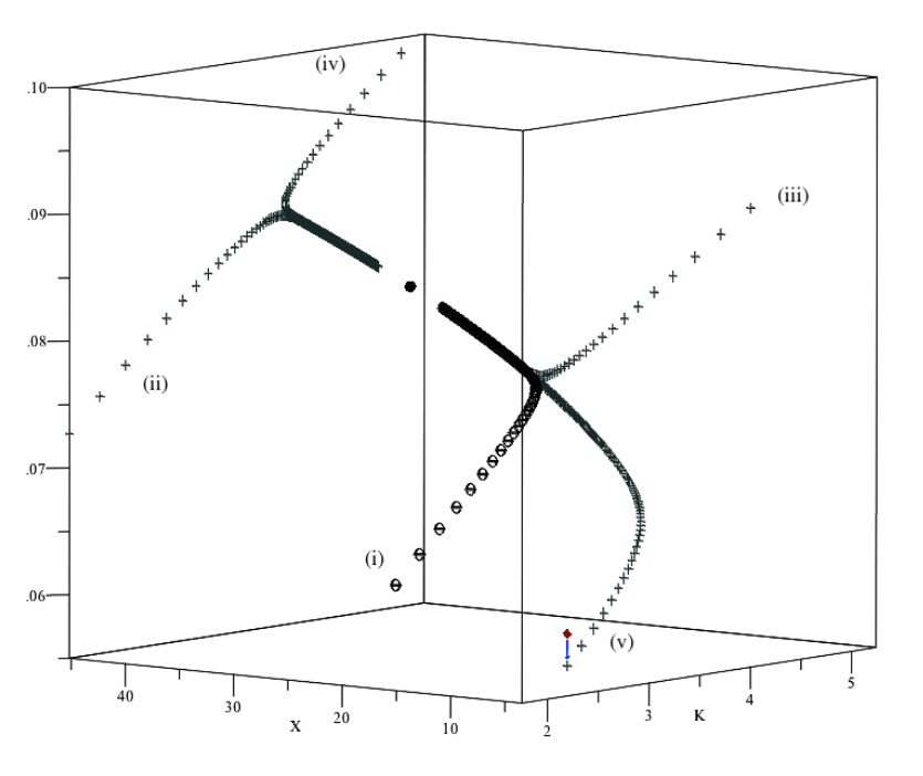
Figure 6. Stable paths.
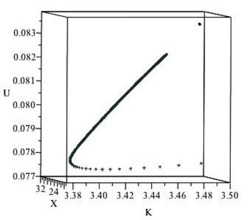
Figure 7. An unsustainable path starting from a small level of capital.
Important policy implications emerge from this framework. Although we did not discuss the manner in which society determines the allocation of resource bases to energy production, we can envision a number of approaches. Society could impose standards that require a certain level of usage of renewables, as with Renewable Performance Standards—popular in some US states. Or society could adopt a tradable permit scheme for carbon emissions, as with the EU's emission trading system. A third option is to invoke a carbon tax—as in the Canadian province of British Columbia—which raises the cost of (non-renewable) fossil fuels. The presence of a capacity constraint on the use of renewables would suggest that none of these policies can induce increased renewable production in the moment (as the capacity constraint would preclude such expansion), though it seems likely to encourage increased investment in renewable capacity—and perhaps research into new innovations [50]). In this regard, the financial rewards associated with avoiding the carbon tax would seem pose an attractive incentive in a decentralized economy, such as that found in most Western countries. In addition, we find that a short period in which renewable energy development is put on hold—as one might envision occurring under the newly elected U.S. President Trump— can cause a dramatic delay in the time it takes to reach long-run equilibrium.
Throughout the paper, we have assumed that felicity is not separable: additional felicity from marginal consumption is directly affected by the stocks of renewable natural capital and pollution. The more society cares about renewable natural capital, the higher is its steady-state value [51]. Moreover, for a non-zero steady-state level of renewable natural capital to exist, society must be sufficiently willing to trade today's consumption for tomorrow's consumption; this can be interpreted as the need for society to be averse to intergenerational inequity. This is because society can only increase the stock of renewable natural capital by reducing energy used in current output production, which lowers both output and consumption today. The non-linear relationship between consumption, pollution and the renewable resource stock imply that none can be analyzed independently, their evolution through time and their long-run values are linked. The time when society starts using renewable energy is determined by the relative magnitude of the shadow price of pollution and the shadow value of each resource stock. The evolution of each of these components is dictated by society's preferences and the initial levels pollution as well as man-made, non-renewable and renewable capital.
Returning to the discussion in section , a necessary condition for sustainability is that the initial levels of and are smaller than their respective steady-state values, e.g., scenario (i). Any trajectory that requires a reduction in one of the state variables is unsustainable, as is any scenario that requires society accept a reduction in output, as when it ends a moratorium on renewable capital accumulation.
6.- Concluding Remarks
In this paper, we investigated the role of energy in sustainability in a model where nonrenewable energy contributes to a pollution stock, and where the use of renewable energy requires the endogenous development of a stock of renewable capital. Societal well-being, or “felicity”, is larger the larger is either consumption of the stock of renewable resources, but is decreasing in the level of pollution: people like to consume and enjoy the environment for all the different kinds of ecological services it supplies, but dislike pollution. Felicity is also assumed to be non-separable in consumption and the remaining renewable resources. Renewable and non-renewable resources are used to generate energy, which can be used to increase the regeneration process of the renewable natural capital, to abate pollution that comes with the use of non-renewable energies or to increase output. Interpreting sustainability as the restriction that felicity never decrease as time goes by, we find that consumption and the stock of renewable natural capital grow faster than the stock of pollution, each weighted by their respective marginal effect on utility.
We illustrate some important properties of the model by use of a numerical simulation. In the example we analyze, it is optimal to completely switch from non-renewable to renewable resources in energy production. This transformation allows energy to be directed away from abatement, which facilitates a perpetual increase in consumption, thereby allowing continual growth in felicity. In the post non-renewables phase, we find that the system dynamics are saddle-path stable in a neighborhood of the steady-state. We also find that the steady-state level of renewable natural capital depends on the society's elasticity of inter-temporal substitution in consumption. We also note that it takes a relatively long time to get close to the renewable natural capital steady-state in our simulation, suggesting that society must take a long view of the resource allocation problem. Finally, we observe that a moratorium on investment in renewable resource capital accumulation is unsustainable, as there will be a reduction in output—followed by a decrease in consumption and felicity—when the moratorium is removed.
References and Notes
| [1] | Pezzey JC, Toman MA. The Economics of Sustainability: A Review of Journal Articles. Washington, DC, USA: Resources for the Future; 2002. Discussion Paper 02–03. |
| [2] | Solow RM. Sustainability: an economist’s perspective. In: Dorfman R, editor. Economics of the Environment: Selected Readings. New York, NY, USA: Norton and Company; 1993. pp. 179–187. |
| [3] | Moe T, Alfsen K, Greaker M. Sustaining Welfare for Future Genera- tions: A Review Note on the Capital Approach to the Measurement of Sustainable Development. Challenges in Sustainability. 2013;1(1):16– 26. doi:10.12924/cis2013.01010016. |
| [4] | Hartwick JM. Intergenerational Equity and the Investing of Rents from Exhaustible Resources. American Economic Review. 1977;67(5):972—974. |
| [5] | Annual Energy Outlook. Washington, DC, USA: U.S. Energy Infor- mation Administration (EIA); 2015. DOE/EIA-0383(2015). Available from: http://www.eia.gov/forecasts/aeo/pdf/0383(2015).pdf. |
| [6] | The US Energy Information Administration [5] lists the levelized cost of electricity (LCOE) for new energy sources to come online in 2020. The LCOE breaks down into capital costs, fixed and variable oper- ations and maintenance (O&M) costs and transmission costs. For wind and solar energies, variable O&M costs are zero while for hy- droelectricity, they only account for 8.4% of the total LCOE. When sunk initial capital costs and fixed O&M costs are combined, they represent from 89% to 98% of the LCOE for renewables (wind, solar and hydro electricity). This compares to less than 35% for the multiple technologies of gas-fired plants, and up to about 74% for newest coal-fired plants. |
| [7] | What is the energy payback for PV? Washington, DC, USA: Na- tional Renewable Energy Laboratory; 2004. DOE/GO-102004-1847. Available from: www.nrel.gov/docs/fy04osti/35489.pdf. |
| [8] | Knapp K, Jester T. An Empirical Perspective on the Energy Payback Time for Photovoltaic Modules. Solar Energy. 2001;71(3):165–172. 8 doi:10.1016/s0038-092x(01)00033-0. |
| [9] | Staffell I, Green R. How Does Wind Farm Performance Decline with Age? Renewable Energy. 2014;66:775–786. doi:10.1016/j.renene.2013.10.041. |
| [10] | Jordan DC, Kurtz SR. Photovoltaic Degradation Rates: An Analyti- cal Review. Progress in Photovoltaics: Research and Applications. 2011;21(1):12–29. doi:10.1002/pip.1182. |
| [11] | Meadows DH, Meadows DL, Randers J, Behrens III W. The Limits to Growth. New York, NY, USA: Universe Books; 1972. |
| [12] | Malthus TR. An Essay on the Principle of Population. New York, NY, USA: Norton; 1976. (Originally published in 1798). |
| [13] | The debate regarding sustainability can be traced back as far as 1798 [12]. For a thorough survey of this literature see [1]. |
| [14] | Nordhaus WD, Stavins RN, Weitzman ML. Lethal Model 2: The Limits to Growth Revisited. Brookings Papers on Economic Activity. 1992;1992(2):1. doi:10.2307/2534581. |
| [15] | Heyes AG, Liston-Heyes C. Sustainable Resource Use: The Search for Meaning. Energy Policy. 1995;23(1):1–3. doi:10.1016/0301- 4215(95)90761-u. |
| [16] | Solow R. An Almost Practical Step toward Sustainability. Resources Policy. 1993;19(3):162–172. doi:10.1016/0301-4207(93)90001-4. |
| [17] | Jevons S. The Coal Question: An Inquiry Concerning the Progress of the Nation and the Probable Exhaustion of Our Coal Mines. 2nd ed. London, UK: Macmillan; 1866. |
| [18] | Forster BA. Optimal energy use in a polluted environment. Journal of Environmental Economics and Management. 1980;7(4):321–333. doi:10.1016/0095-0696(80)90025-x. |
| [19] | Withagen C. Pollution and exhaustibility of fossil fuels. Resource and Energy Economics. 1994;16(3):235–242. doi:10.1016/0928- 7655(94)90007-8. |
| [20] | Tahvonen O. Fossil Fuels, Stock Externalities, and Backstop Tech- nology. The Canadian Journal of Economics. 1997;30(4a):855. doi:10.2307/136274. |
| [21] | Jouvet PA, Schumacher I. Learning-by-doing and the costs of a back- stop for energy transition and sustainability. Ecological Economics. 2012;73:122–132. doi:10.1016/j.ecolecon.2011.10.007. |
| [22] | Tahvonen O, Salo S. Economic growth and transitions between renew- able and nonrenewable energy resources. European Economic Review. 2001;45(8):1379–1398. doi:10.1016/s0014-2921(00)00062-3. |
| [23] | van der Ploeg F, Withagen C. Growth, Renewables and the Optimal Carbon Tax. International Economic Review. 2014;55(1):283–311. doi:10.1111/iere.12049. |
| [24] | This approach is in line with the most prevalent approach used by economists. The numerical results from such an approach are useful in characterizing broad trends and policy implications. This approach is very different to agent-based models and models of the MARKAL family. Agent-based modeling is useful when modeling interactions at an individual-level with multiple agents and allows to capture many institutional details; such a framework necessitates high computing power to yield aggregate behavior. However, in the case of a first-best solution with a representative agent, agent-based modeling would add an unnecessary level of complexity and would not yield additional valuable results. MARKAL models use a stylized representation of an energy production system to simulate various policies; in this way, they are similar to Integrated Assessment Models (IAM). While MARKAL models and IAMs consider a range of variables, they are difficult to generalize. |
| [25] | We adopt the notation to denote the time derivative of a variable. |
| [26] | This approach is similar to the concept of energy payback from lifecy- cle analysis. For instance, the National Renewable Energy Laboratory lists payback times—how long a unit has to operate to offset the to- tal energy used to manufacture the system—for photovoltaics to be between 1 and 3.3 years [7]. Knapp and Jester [8] check estimate that, depending on the technology, between 3 MWh to 16.5 MWh are necessary to produce a 1 kW solar panel. |
| [27] | Zilberman D, Barrows G, Hochman G, Rajagopal D. On the Indi- rect Effect of Biofuel. American Journal of Agricultural Economics. 2013;95(5):1332–1337. doi:10.1093/ajae/aat038. |
| [28] | This depreciation can be substantial. For example, Staffel and Green [9] find that for wind farms in the United Kingdom , load factors—the percentage of electricity actually produced, compared to the theoreti- cal maximum—falls by roughly 1.5% per year. While less dramatic, depreciation rates for solar photovoltaics are on the order of 0.5% per year [10]. |
| [29] | For example, oil sands extraction in Alberta, Canada leaves signif- icant tailings, in particular containment ponds retaining water with fine or toxic residues. Environmental regulations require industry to restore the extraction site to its pre-extraction state. |
| [30] | See http://www.garbagepatchstate.org. We note that most plastics are made from petrochemicals. |
| [31] | One could also think of the renewable resource as bio-energy, whose stock naturally grows in relation to the stock level, but is diminished by harvesting [27]. In that setting, one can think of energy as being used to increase the capability of a facility to generate bio-fuels. |
| [32] | Stern N. The Economics of Climate Change: The Stern Review. Cambridge, UK: Cambridge University Press; 2007. |
| [33] | Nordhaus W. Economics: Critical Assumptions in the Stern Review on Climate Change. Science. 2007;317(5835):201–202. doi:10.1126/science.1137316. |
| [34] | This discount rate was the source of considerable controversy in the context of climate policy. For example, Stern proposes a very low discount rate, barely positive [32], while Nordhaus suggests a rate closer to 3% [33]. |
| [35] | Mason CF, Chass´ e RM. The Switch to Renewable Energy. Laramie, WY, USA: University of Wyoming; 2017. Department of Economics Working Paper. |
| [36] | Technical details of our analysis, and mathematical derivations, are available in a companion paper [35]. |
| [37] | Xepapadeas A. Economic Growth and the Environment. In: M¨ alex K, Vincent J, editors. Handbook of Environmental Economics. Vol. 3. Amsterdam, The Netherlands: Elsevier; 2003. pp. 1219–1271. |
| [38] | Following Xepapadeas [37]. Felicity can be either separable non- separable in and . Separable utility would imply that an increase in pollution would have no effect on the marginal felicity from con- sumption or from the stock of renewable resource (because the cross- partial derivatives between consumption and both and would then be zero). While this facilitates analytical tractability, it precludes some important features in terms of how renewable resource capital and pollution affect felicity and marginal utility from consumption. Because our analysis relies on simulations, as opposed to seeking analytical closed-form solutions, we prefer to use a non-separable utility formulation. |
| [39] | Hansen LP, Singleton KJ. Generalized Instrumental Variables Esti- mation of Nonlinear Rational Expectations Models. Econometrica: Journal of the Econometric Society. 1982;50(5):1269–1286. |
| [40] | Assuming an exponent of 0.5 on consumption implies the inter- temporal elasticity of substitution equals 2. This parameter in- dicates how willing society is to substitute current consumption for consumption in the future: larger values imply greater societal will- ingness to smooth consumption over time. Our choice is consistent with Tahvonen and Sallo [22], who require . In Hansen and Singleton [39], ranges from 1.05 to 1.47, while in van der Ploeg and Withagen (2014) = 0.5. A referee points out that the utility function we use in the numerical simulations is not well defined at zero pollution stock, and that the pollution stock tends to zero in the infinite limit. This poses no difficulties in the numerical application, as we simulate for a finite number of periods; to avoid the problem in the conceptual analysis, one could add an arbitrarily small positive value to stock (which might be interpreted as a “pre industrial” level). For a suitably small value, such a refinement would not change the simulation results, though it would complicate the presentation. |
| [41] | While some renewable energies are perfect substitutes to non- renewable energies, there are some potential difficulties in substitu- tion. For example, renewable energy production is subject to intermit- tency due to meteorological uncertainties, while energy production from coal is not. By assuming the resources are perfect substitutes, we are implicitly assuming that these issues can be overcome. |
| [42] | In economic parlance, “the shadow values” of the two types of natural capital become equal at time . In these simulations, 1.87; inter- preting a period as one year, this corresponds to roughly 20 months. |
| [43] | In a steady-state, the different state (man-made and renewable capi- tal) and control (renewable resource use, consumption and energy shares) variables stop changing, i.e., . Several other variables also stop changing once a steady-state has been reached: . Here, for the steady- state value of the renewable resource stock to be positive, the repre- sentative agent must be averse to intergenerational inequality. |
| [44] | As the system of equations is non-linear, one usually would proceed by linearizing around the steady-state; this allows analysis of the be- havior of the system close to the equilibrium point. Here, the system is saddle-point stable. |
| [45] | We assume , whereas in the simulation. Because renewable capital is procured via investment, one would expect the initial level to lie below the steady-state value. Accordingly, scenarios (iii) and (iv) are unlikely to be empirically plausible; we include them solely for the sake of completeness. |
| [46] | Interestingly, as soon as this policy is adopted, it takes just about 2 years to achieve the same level of felicity as before. |
| [47] | Note that at would imply the elasticity of substi- tution between renewable and non-renewable resources could not equal unity; in turn, this would preclude the use of a Cobb-Douglas function to model energy generation. |
| [48] | Vardar NB. Imperfect resource substitution and optimal transition to clean technologies. Universit´ e Catholique de Louvain; 2013. CORE discussion paper 2013/72. Available from: http://www.uclouvain.be/ cps/ucl/doc/core/documents/coredp2013 72web.pdf. |
| [49] | This calls to mind the quote from Sheik Yamani, former oil minister for OPEC: “[t]he stone age did not end for lack of rocks, and the oil age will not end for lack of oil”. |
| [50] | Acemoglu D, Aghion P, Bursztyn L, Hemous D. The Environ- ment and Directed Technical Change. American Economic Review. 2012;102(1):131–166. doi:10.1257/aer.102.1.131. |
| [51] | This is a consequence of a increase in parameter ˜ b in the utility function. 10 |
Continue reading the article
This document is for reference purposes only. It does not replace the original published article in PDF format and in no way shall be interpreted or considerate to create any warranties of any kind, please refer to the [formal published version] as a source for a reference.
For more information visit our digital information page.